Part 4: Rosenblatt’s Perceptron: How the First Trainable Neural Network Was Created

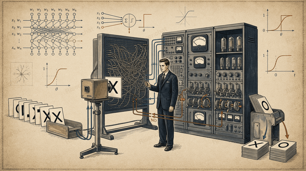
Table of Contents

1. What Is a Perceptron? A Short Answer
2. How the Perceptron Differed from the McCulloch–Pitts Model
3. Who Was Frank Rosenblatt?
4. How a Perceptron Works in Simple Terms
5. Traditional Programming and Machine Learning
6. The Main Components of a Perceptron
7. The Perceptron Learning Algorithm
8. How a Perceptron Corrects an Error
9. What Does It Mean to Say That a Perceptron Learned?
10. How a Perceptron Makes a Decision
11. The Perceptron Convergence Theorem
12. How Rosenblatt’s Historical Perceptron Was Designed
13. What Was the Mark I Perceptron?
14. What Could the Mark I Perceptron Do?
15. Why the Perceptron Caused So Much Excitement
16. Did Rosenblatt Promise to Create Artificial Intelligence?
17. What Is a Single-Layer Perceptron?
18. What Problems Can a Simple Perceptron Solve?
19. Why a Single-Layer Perceptron Cannot Solve XOR
20. Other Limitations of the Perceptron
21. The Perceptron and the Criticism of Minsky and Papert
22. Was the Perceptron the First Trainable Neural Network?
23. The Perceptron and Modern Neural Networks
24. How the Perceptron Is Connected to Deep Learning
25. How the Perceptron Is Connected to ChatGPT and Claude
26. Why the Perceptron Is Still Studied
27. A Brief History of the Perceptron
28. Key Concepts
29. Frequently Asked Questions
30. Conclusion

---

Modern neural networks recognize images, translate texts, analyze documents, write software code, and hold conversations. AI models such as ChatGPT and Claude may contain billions of parameters and be trained on enormous datasets.

Yet one of the most important steps toward modern artificial intelligence was taken long before the internet, graphics processing units, and large language models existed.

In the late 1950s, American psychologist Frank Rosenblatt proposed the perceptron—a neural network model capable of changing its parameters after making mistakes.

Researchers no longer had to define every classification rule manually. The machine was shown examples and given the correct answers, after which it gradually adjusted the connections between its components.

The perceptron did not understand images the way a human does. It could not talk, write texts, or reason. Nevertheless, it already contained the principle that would later become the foundation of a large part of machine learning:

A system can improve its results by changing its internal parameters based on experience.

This idea paved the way from the first mathematical neurons to deep neural networks and, eventually, to modern artificial intelligence systems.

What Is a Perceptron? A Short Answer

A perceptron is a simple trainable artificial neural network model. It receives input data, multiplies the inputs by weights, adds the results together, and chooses one of two possible answers. If the answer is wrong, the algorithm adjusts the weights.

After this process is repeated many times, the perceptron can learn to separate objects into two classes.

Its basic workflow looks like this:

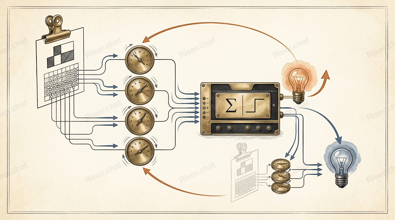
input features → weights → weighted sum → threshold → output → error check → weight update.

For example, a perceptron can be trained to distinguish cards with a mark on the left from cards with a mark on the right. At first, the model’s answers are nearly random. After every incorrect response, it changes its parameters and gradually discovers a pattern that separates the two types of images.

Rosenblatt’s perceptron is often called the first trainable neural network. A more precise description is that it became one of the first widely known and practically implemented neural network systems capable of learning classification from examples.

Mathematical models of artificial neurons and early experimental machines had already existed before it. However, the perceptron brought together several key elements:

• a neural network structure;
• learning from errors;
• a mathematical foundation;
• the ability to generalize;
• software and hardware implementations.

---

How the Perceptron Differed from the McCulloch–Pitts Model

In 1943, Warren McCulloch and Walter Pitts proposed a formal model of an artificial neuron.

This neuron received binary signals, compared their sum with a threshold, and produced one of two outputs: 0 or 1. A network made from such elements could perform logical operations.

However, its connections, thresholds, and structure had to be defined by a researcher in advance. The model did not analyze its own mistakes or change after receiving a new example.

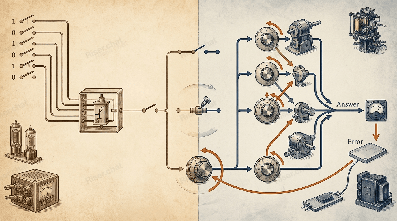
The perceptron added a fundamentally new capability: learning.

McCulloch–Pitts model	Rosenblatt’s perceptron
Proposed in 1943	Developed in the 1950s
Describes a threshold-based artificial neuron	Describes a trainable recognition system
Connections are predefined	Some connections can change
Does not use errors for learning	Adjusts weights after errors
Executes a predefined function	Finds a classification rule from examples
Primarily a theoretical model	Implemented in both software and hardware

The main difference can be explained in simple terms:

The McCulloch–Pitts model executed a rule created by a person, while the perceptron could derive part of that rule from training examples.

This did not mean that the machine learned without human involvement. A person still had to:

• define the problem;
• choose the system architecture;
• prepare the input data;
• provide the correct answers;
• configure the learning parameters;
• launch and supervise the experiment.

However, the exact values of the adjustable weights no longer had to be calculated manually.

McCulloch and Pitts demonstrated how an artificial neural network could perform computations. Rosenblatt took the next step and demonstrated how such a system could change under the influence of experience.

---

Who Was Frank Rosenblatt?

Frank Rosenblatt was an American psychologist and researcher who worked at the intersection of psychology, neurophysiology, mathematics, and computer science.

He was born in New York in 1928 and studied psychology at Cornell University, where he later earned his doctoral degree.

Rosenblatt was interested in more than simply programming a computer to perform a specific task. He wanted to understand broader mechanisms:

• how living organisms perceive the world around them;
• how the brain stores information;
• how previous experience affects new decisions;
• how people learn to recognize similar objects;
• whether certain properties of perception could be reproduced in a machine.

After earning his doctorate, Rosenblatt worked at the Cornell Aeronautical Laboratory in Buffalo. It was there that he began developing the theory of perceptrons.

He viewed the perceptron not merely as a computer program, but as a simplified model of the nervous system. He was interested in whether learning, memory, and perception could be explained through the operation of many interconnected elements.

This approach later became known as connectionism. Its central idea is that knowledge is not stored as a single ready-made rule but distributed across many connections within a network.

Rosenblatt described an early version of the perceptron in 1957. In November 1958, his paper The Perceptron: A Probabilistic Model for Information Storage and Organization in the Brain was published in Psychological Review. The paper presented the perceptron as a probabilistic model for storing and organizing information.

In 1962, Rosenblatt summarized his research in the book Principles of Neurodynamics: Perceptrons and the Theory of Brain Mechanisms.

It is important to understand that Rosenblatt’s theory was much broader than the modern classroom example involving a single output neuron. He examined various architectures, including more complex, multilayer, and cross-coupled systems.

Nevertheless, the best-known part of his legacy is the simple single-layer perceptron—a linear classifier that learns from errors.

The development of the perceptron and its early demonstration on the IBM 704 are described in detail in Cornell University’s archival materials.

---

How a Perceptron Works in Simple Terms

Imagine that we need to create a system that determines whether an email is spam.

Each email can be described using several features:

• whether it contains the word “prize”;
• whether the subject line is written in capital letters;
• whether the email contains a suspicious link;
• whether the sender is unknown;
• whether the message contains many exclamation marks.

For a perceptron, each feature is converted into a number.

For example:

• the feature is present—1;
• the feature is absent—0.

Every input has its own weight. A weight indicates how strongly a particular feature influences the final decision.

If suspicious links frequently appear in spam messages, the corresponding weight may become large and positive. If the email was sent by a known sender, that feature may instead reduce the likelihood of the message being classified as spam.

The perceptron performs several operations:

1. receives numerical features;
2. multiplies each feature by its weight;
3. adds the resulting values together;
4. adds a bias;
5. compares the result with a threshold;
6. produces an output of 0 or 1.

Mathematically, this can be written as:

S = x₁w₁ + x₂w₂ + ... + xₙwₙ + b

Where:

• x is an input feature;
• w is the feature’s weight;
• b is the bias;
• S is the weighted sum.

A threshold rule is then applied:

• if S ≥ 0, the output is 1;
• if S < 0, the output is 0.

In our example:

• 1 may mean “spam”;
• 0 may mean “regular email.”

At first, the weights may be zero or random, so the model will make mistakes. It is then shown the correct answer.

If an email is actually spam but the perceptron classifies it as a regular message, the algorithm changes the weights. Features associated with spam begin to have a stronger effect on future decisions.

This is how learning occurs:

The model is not given a ready-made verbal rule. Instead, it adjusts numerical parameters based on examples.

---

Traditional Programming and Machine Learning

Before trainable models appeared, computer problems were usually solved through explicit instructions.

Traditional Programming

A developer provides the data and the rules:

data + rules → result.

For example:

If the subject line contains the word “prize”
and the sender is unknown,
mark the message as spam.

The program executes a rule formulated by a person.

Machine Learning

A developer provides examples and correct answers:

data + correct answers → model configuration.

For example:

Email 1 — spam.
Email 2 — not spam.
Email 3 — spam.
Email 4 — not spam.

The algorithm independently adjusts the weights that make it possible to separate the two classes.

Of course, modern machine learning is far more complex than a simple perceptron. Specialists still define the model architecture, prepare the data, select the loss function, and configure the training process.

However, the shift from manually describing every rule to adjusting parameters based on data became one of the most important changes in the history of artificial intelligence.

Modern neural networks follow the same general principle: much of a model’s knowledge is represented not as individual commands but as a large collection of numerical parameters.

---

The Main Components of a Perceptron

In a simplified representation, a perceptron consists of six main components.

Input Values

The inputs describe the object that needs to be classified:

x = (x₁, x₂, ... xₙ).

For a black-and-white image, the inputs may be pixels:

• white pixel—0;
• black pixel—1.

For text data, the inputs may indicate the presence of certain words or symbols. For physical measurements, they may represent temperature, mass, speed, or object size.

The perceptron does not understand the physical meaning of these features. To the model, every object is simply a set of numbers.

Weights

Each input has a corresponding weight:

w = (w₁, w₂, ... wₙ).

A weight determines how a feature influences the decision:

• a positive weight supports class 1;
• a negative weight supports class 0;
• a weight close to zero means that the feature has little influence on the result.

The weights are the parameters that change during training.

Weighted Sum

The inputs are multiplied by their weights and added together:

S = x₁w₁ + x₂w₂ + ... + xₙwₙ + b.

The larger the sum, the more strongly the combination of features supports class 1.

Bias

The parameter b is called the bias. It allows the decision boundary to move independently of specific input values.

Historical descriptions often use a threshold instead of a bias:

x₁w₁ + x₂w₂ + ... + xₙwₙ ≥ θ.

Both forms express the same basic idea: the model compares the weighted sum with a particular boundary.

Threshold Function

The sum is converted into one of two outputs:

• y = 1 if S ≥ 0;
• y = 0 if S < 0.

The classic perceptron uses an abrupt threshold switch. Modern neural networks often use smoother activation functions that are more suitable for training multilayer models.

Correct Label and Error

Every training example has a correct answer, represented by t.

The error is calculated as:

e = t − y.

Three situations are possible:

• e = 0—the model produced the correct answer;
• e = 1—the model should have produced 1 but produced 0;
• e = −1—the model should have produced 0 but produced 1.

The sign of the error determines the direction in which the weights need to be changed.

---

The Perceptron Learning Algorithm

Perceptron training can be divided into six steps.

Step 1: Initialize the Weights

First, the weights and bias are assigned initial values.

For example:

• w₁ = 0;
• w₂ = 0;
• b = 0.

Small random numbers may also be used.

Step 2: Provide a Training Example

The model receives an object:

x = (x₁, x₂, ... xₙ).

The correct label t is provided along with it.

Step 3: Calculate the Output

The perceptron calculates the sum:

S = w₁x₁ + w₂x₂ + ... + wₙxₙ + b.

It then applies the threshold function and obtains the prediction y.

Step 4: Calculate the Error

The prediction is compared with the correct answer:

e = t − y.

If the error is zero, the parameters remain unchanged.

Step 5: Update the Weights

If the model makes a mistake, the weights are adjusted:

wᵢ ← wᵢ + η(t − y)xᵢ

The bias is updated in a similar way:

b ← b + η(t − y)

Here, η is the learning rate.

It determines the size of each update:

• with a small value, the weights change slowly;
• with a large value, they change more sharply.

If a particular input is zero, its corresponding weight will not change during that step. If the input is active, the direction of the update depends on the sign of the error.

Step 6: Repeat the Process

The model receives the next example, makes another prediction, and changes its parameters if necessary.

One complete pass through the training dataset is called an epoch. If errors remain, another epoch begins with the updated weights.

The general process looks like this:

example → prediction → correct answer → error → weight update → new example.

Modern neural networks, including the models behind ChatGPT and Claude, are trained using far more complex methods. Nevertheless, the same familiar logic remains: the model produces a prediction, an error is calculated, and the parameters are changed to improve future results.

---

How a Perceptron Corrects an Error

Consider a model with two inputs:

• x₁ = 1;
• x₂ = 1.

Suppose the initial parameters are zero:

• w₁ = 0;
• w₂ = 0;
• b = 0.

The correct answer is:

t = 0.

The perceptron calculates the sum:

S = 1 × 0 + 1 × 0 + 0 = 0.

According to the selected rule, when S ≥ 0, the model produces:

y = 1.

This answer is incorrect:

e = t − y = 0 − 1 = −1.

Let the learning rate be:

η = 1.

We update the parameters:

w₁ ← 0 + 1 × (−1) × 1 = −1

w₂ ← 0 + 1 × (−1) × 1 = −1

b ← 0 + 1 × (−1) = −1

If we provide the same example again, we get:

S = 1 × (−1) + 1 × (−1) − 1 = −3

The output is now:

y = 0.

The prediction matches the correct label.

This is an elementary example, but it reveals the central idea:

An error is not merely recorded—it is used to change the model’s future behavior.

The perceptron does not store a verbal explanation of why its first answer was wrong. The result of learning is represented by the new values of the weights and bias.

---

What Does It Mean to Say That a Perceptron Learned?

The phrase “the machine could learn” can easily create the wrong impression.

The perceptron was not conscious and did not understand the meaning of its task. It did not independently decide what to study, nor did it search the outside world for data.

Learning referred to a much narrower mathematical process:

1. the system received an example;
2. it calculated an answer;
3. it received the correct label;
4. it determined the error;
5. it changed numerical parameters;
6. it applied the updated parameters to future examples.

This approach is called supervised learning because the correct answers are known in advance.

The supervisor may be:

• a person;
• another program;
• a pre-labeled dataset;
• an automated example-generation system.

A perceptron does not necessarily memorize every object as a separate rule. Its task is to find a general boundary between two classes.

If the trained model correctly processes a new object that it has never seen before, this is called generalization.

The ability to work with new data rather than merely reproduce answers for training examples remains one of the central goals of machine learning.

---

How a Perceptron Makes a Decision

From a mathematical perspective, a single-layer perceptron is a linear classifier.

Suppose each object is described by two features:

• x₁;
• x₂.

The decision boundary is defined by the expression:

w₁x₁ + w₂x₂ + b = 0.

On a graph, this boundary is a straight line.

Objects on one side of the line are assigned to class 0, while objects on the other side are assigned to class 1.

With three features, the boundary becomes a plane. With more features, it becomes a hyperplane.

During training, the perceptron changes the weights and bias. Geometrically, this can be imagined as the model gradually moving and rotating a line in an attempt to separate the two classes correctly.

If a single straight line can be drawn between red and blue points so that points of different colors appear on opposite sides, the data is called linearly separable.

A simple perceptron can find a suitable boundary for this kind of data.

If the classes are arranged in a more complicated way and one straight line is not enough, a single-layer model cannot classify every example without error.

---

The Perceptron Convergence Theorem

The perceptron is associated with an important mathematical result known as the convergence theorem.

In simplified terms, it states:

If the training data is linearly separable, the perceptron algorithm will find a boundary that correctly separates all training examples after a finite number of updates.

This does not mean that the algorithm will find the only possible boundary or the best boundary among all available solutions. Several valid solutions may exist.

The theorem also does not guarantee successful training for every possible dataset.

If the classes cannot be separated by a single linear boundary, the perceptron may continue changing its weights, moving from one error to another.

Nevertheless, the theorem was highly significant in the history of machine learning. It demonstrated that model training was not merely a random search through parameters. Under certain conditions, it was mathematically possible to prove that the algorithm would reach a correct solution.

---

How Rosenblatt’s Historical Perceptron Was Designed

Modern textbooks often depict a perceptron as a single artificial neuron with several inputs.

This is a useful diagram, but Rosenblatt’s historical model was more complex. He described three main types of elements:

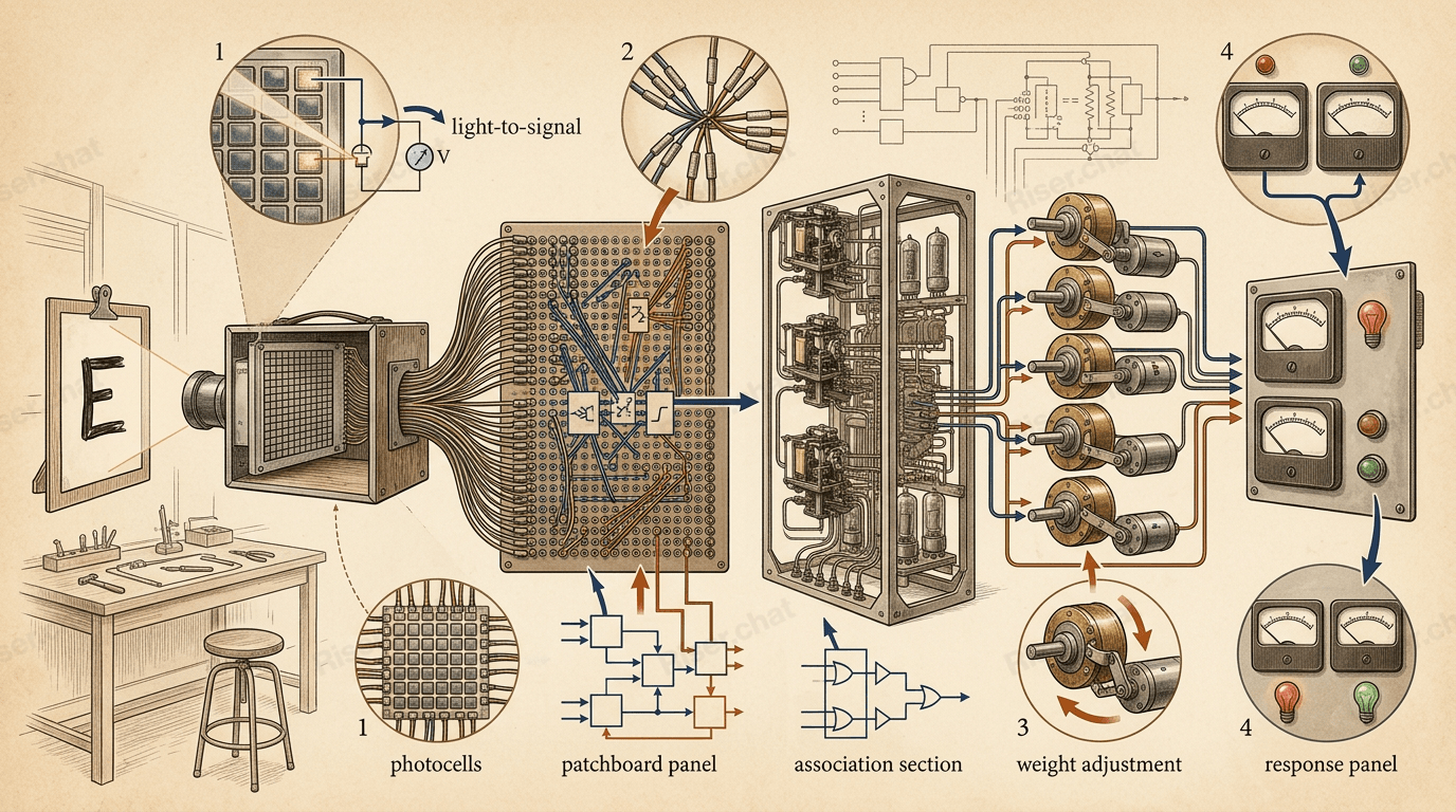
1. S-units—sensory units;
2. A-units—association units;
3. R-units—response units.

Sensory Units

S-units received signals from the external environment.

In an image-recognition system, they acted as a primitive electronic retina and responded to light and dark areas.

Association Units

A-units combined signals from the sensory part of the system.

They could respond not only to an individual pixel but also to combinations of several input features.

Response Units

R-units produced the output response.

One unit could represent the first class, while another represented the second. The result depended on the activity of the output units and the strength of the connections leading to them.

A simplified historical diagram looked like this:

image → sensory units → association units → adjustable connections → output response.

For this reason, the real Mark I Perceptron should not be imagined as a single modern software neuron. It was an experimental electronic machine that implemented individual parts of Rosenblatt’s much broader theory.

The division into sensory, association, and response units is presented in the Smithsonian National Museum of American History’s description.

---

What Was the Mark I Perceptron?

The Mark I Perceptron was a hardware machine created by Rosenblatt’s team at the Cornell Aeronautical Laboratory with support from the U.S. Office of Naval Research and the Rome Air Development Center.

The first experiments were conducted using computer simulations. In July 1958, the algorithm was demonstrated on an IBM 704—a large computer that occupied a considerable part of a room.

During the demonstration, the computer learned to distinguish cards with a mark on the left from cards with a mark on the right. After a series of attempts, the system managed to identify a classification rule.

Researchers later built a specialized physical machine. The Smithsonian National Museum of American History dates the Mark I Perceptron to 1958.

The system included:

• a photosensitive array;
• 400 input signals;
• a patch panel;
• association units;
• adjustable potentiometers;
• output units;
• measuring instruments.

The Mark I camera used a 20 × 20 array of photosensitive elements. An image was converted into 400 input signals, which were then transmitted to the next parts of the machine. The device and its operating principles are also explained in Cornell University’s educational materials.

The patch panel made it possible to change the connections and experiment with different feature sets.

The potentiometers represented adaptive weights. Their physical states determined how strongly individual connections affected the output.

In modern neural networks, weights are stored in computer memory as numbers. In the Mark I, some parameters existed as the physical states of real electronic and electromechanical components.

Learning did not happen only by changing numbers in software—the network’s parameters were physically embodied inside the machine.

The Mark I consisted of several large cabinets. The surviving system is now part of the collection of the Smithsonian National Museum of American History.

---

What Could the Mark I Perceptron Do?

The main purpose of the Mark I was to recognize and classify simple visual patterns.

The machine was shown images or cards containing marks. Its photosensitive array converted each image into a set of signals, after which the system attempted to assign it to one of the available classes.

If the answer was incorrect, the adjustable connections were modified.

This process was a distant early version of modern image classification:

1. the system receives an image;
2. the image is converted into numbers;
3. numerical features pass through the network;
4. the model selects a category;
5. the correct answer is used for training.

The difference was in complexity and scale.

A modern computer vision neural network may contain millions or billions of parameters and may be trained on enormous image datasets. The Mark I received an image represented by only 400 input elements and solved limited experimental tasks.

The Mark I Could

• receive optical signals;
• convert images into numerical inputs;
• classify simple patterns;
• modify some of its internal connections;
• improve its answers through training;
• apply a learned rule to similar examples.

The Mark I Could Not

• understand the meaning of what it saw;
• recognize arbitrary objects in the real world;
• collect training data independently;
• choose its own learning objective;
• hold a conversation;
• reason;
• solve problems involving complex nonlinear relationships;
• operate on the scale of modern artificial intelligence systems.

Nevertheless, the Mark I proved something essential: a trainable neural network could exist not only as a mathematical concept but also as a functioning physical machine.

---

Why the Perceptron Caused So Much Excitement

In the 1950s, computers were generally viewed as fast calculating machines.

They could:

• add numbers;
• calculate trajectories;
• process tables;
• sort data;
• execute a programmer’s instructions.

The perceptron appeared to be different. Its creators did not directly specify the final classification rule. The machine changed its behavior after receiving new examples.

To the general public, this looked almost like the birth of an electronic mind.

The appearance of the machine made an even stronger impression. Its large cabinets, wired panels, photosensitive “retina,” instruments, and adjustable components resembled technology from science fiction.

Military agencies were also interested in automated image recognition. Such systems could potentially be used to analyze aerial photographs, detect objects, and process signals.

In July 1958, the perceptron demonstration received widespread coverage in the American press.

One of the best-known reports appeared in The New York Times on July 8, 1958, under the headline New Navy Device Learns by Doing.

Media reports discussed extraordinarily bold expectations. It was suggested that future machines of this kind might be able to see, read, write, speak, and display other abilities associated with human intelligence.

Today, this pattern feels familiar. A similar sequence appears during almost every new artificial intelligence boom:

1. researchers demonstrate a genuine technical achievement;
2. the press extends it to a much broader range of tasks;
3. a limited experiment is transformed into a promise of universal intelligence;
4. expectations begin growing faster than the technology’s actual capabilities.

The perceptron was indeed an important achievement. However, the public often perceived it not as an early classifier but as an almost complete thinking machine.

---

Did Rosenblatt Promise to Create Artificial Intelligence?

Frank Rosenblatt was an optimistic researcher who genuinely viewed perceptrons as a path toward more complex systems of perception, memory, and behavior.

However, three different things must be distinguished:

• the capabilities of the actual Mark I machine;
• Rosenblatt’s broader scientific program;
• sensational newspaper predictions.

Rosenblatt was not studying only a system that distinguished between cards. He was attempting to create a general theory of learning machines inspired by the structure of the brain.

His predictions therefore applied more to the future development of an entire class of systems than to the capabilities of a single hardware installation.

That distinction often disappeared in public reporting.

The statement “the system can adjust its weights after an error” was transformed into “the machine can think.”

In reality, there was an enormous gap between those two abilities. Bridging it required:

• more sophisticated architectures;
• effective methods for training multiple layers;
• powerful computing hardware;
• large digital datasets;
• new activation functions;
• a more advanced theory of optimization.

Decades of research were required before neural networks could reliably recognize objects, process natural language, and generate coherent text.

---

What Is a Single-Layer Perceptron?

A single-layer perceptron is a model in which input values are directly connected to output units, with no trainable hidden layer between them.

A simplified diagram looks like this:

inputs → trainable weights → output.

The input set is sometimes called the input layer. However, it is often excluded when computational layers are counted because it does not perform a separate transformation on its own.

If there is one output, the perceptron solves a binary classification problem:

• 0—regular email;
• 1—spam.

If there are several output units, each may correspond to a separate category.

The defining feature of a single-layer perceptron is that it creates a linear boundary. As a result, it works only with problems in which the classes can be separated by a line, plane, or hyperplane.

---

What Problems Can a Simple Perceptron Solve?

A perceptron can perform logical operations when the corresponding data is linearly separable.

Logical AND

The AND operation returns 1 only when both inputs are equal to 1.

x₁	x₂	x₁ AND x₂
0	0	0
0	1	0
1	0	0
1	1	1

The combination (1, 1) can be separated from the other three points by a single straight line.

Logical OR

The OR operation returns 1 if at least one input is active.

x₁	x₂	x₁ OR x₂
0	0	0
0	1	1
1	0	1
1	1	1

The point (0, 0) can also be separated using a single straight line.

Simple Classification

A perceptron is suitable for problems in which a combination of features consistently separates one class from another.

This may include classification based on:

• size;
• brightness;
• mass;
• temperature;
• the presence of a particular property;
• the frequency of a word or symbol;
• a set of binary features.

However, the model’s capabilities are always limited by the geometry of the data.

---

Why a Single-Layer Perceptron Cannot Solve XOR

The most famous limitation of the perceptron is associated with XOR, or “exclusive OR.”

It returns 1 when exactly one of the two inputs is active.

x₁	x₂	x₁ XOR x₂
0	0	0
0	1	1
1	0	1
1	1	0

If the four combinations are plotted on a graph, points belonging to the same class appear in opposite corners.

It is impossible to draw a single straight line that separates both class 1 points from both class 0 points.

The perceptron can change its weights indefinitely, but every linear boundary will misclassify at least one example.

The problem is not insufficient training time or poor initial values.

For a single-layer linear model, a correct solution simply does not exist.

A simple perceptron can learn only a linearly separable function.

XOR can be implemented using multiple artificial neurons if an intermediate, or hidden, layer is added. Several boundaries working together can form a more complex decision region.

However, in the 1950s and 1960s, there was no sufficiently convenient and universal method for training multilayer neural networks.

---

Other Limitations of the Perceptron

XOR became the best-known example, but the limitations of the single-layer perceptron do not end there.

Only a Linear Boundary

A single perceptron divides feature space using one hyperplane.

If objects from one class form several separate regions or are surrounded by objects from another class, a single line is not enough.

A Hard Binary Output

The classic perceptron produces either 0 or 1.

It does not produce a well-calibrated probability or indicate how confident it is in the answer.

Dependence on Input Features

The model can work only with the features it receives.

If a useful pattern is not represented linearly in the original data, the perceptron cannot independently create a complex internal representation.

In a deep neural network, hidden layers gradually extract more abstract features. A classic single-layer perceptron does not have this capability.

No Convergence on Nonseparable Data

If the training examples cannot be separated by one line, the algorithm may continue changing the weights without ever reaching a final solution.

Real-world data often contains:

• noise;
• measurement errors;
• overlapping classes;
• incorrect labels;
• ambiguous examples.

Limited Computing Resources

The Mark I was an impressive machine for its time, but increasing the number of inputs, connections, and trainable elements quickly made its physical construction more complicated.

No Effective Training for Deep Layers

Adding more layers could theoretically expand the capabilities of a neural network, but it created a difficult question:

How can we determine which internal connection is responsible for an error at the output?

This problem was later addressed using backpropagation and gradient-based methods.

Without an effective way to train multilayer networks, modern computer vision systems, transformers, ChatGPT, Claude, and other large neural models could not have been created.

---

The Perceptron and the Criticism of Minsky and Papert

In 1969, Marvin Minsky and Seymour Papert published Perceptrons: An Introduction to Computational Geometry.

The authors conducted a detailed mathematical analysis of the capabilities and limitations of certain classes of perceptrons.

The book is often described as a work that proved all neural networks were useless. That is an overly crude simplification.

Minsky and Papert analyzed specific types of systems and showed that single-layer models could not solve a number of problems. They understood that multilayer architectures could theoretically possess broader capabilities.

The problem was different: no effective and convenient method for training those networks existed at the time, while computing resources remained extremely limited.

As a result, mathematically justified criticism coincided with disappointment caused by inflated expectations.

Funding for neural network research declined, and many researchers shifted their attention to symbolic artificial intelligence.

However, neural network research did not disappear. Work continued, and interest in multilayer networks began to recover during the 1980s.

The criticism of the perceptron, the XOR problem, and the first AI winter will be covered in greater detail in the next article in this series.

---

Was the Perceptron the First Trainable Neural Network?

The answer depends on how we define a neural network and learning.

Before the perceptron, there were already:

• the McCulloch–Pitts artificial neuron model;
• Hebb’s rule for modifying connections;
• the SNARC neural network machine created by Marvin Minsky and Dean Edmonds;
• research into adaptive and self-organizing systems;
• early learning and recognition models.

It would therefore be inaccurate to claim that no trainable system existed before Rosenblatt’s work.

However, the perceptron combined several important elements:

• a neural network architecture;
• automatic adjustment of connections;
• learning from labeled examples;
• mathematical analysis;
• the ability to generalize;
• computer simulation;
• specialized hardware implementation;
• a public demonstration.

The most accurate description is therefore:

Rosenblatt’s perceptron became one of the first widely known and practically implemented neural networks capable of learning classification from errors.

---

The Perceptron and Modern Neural Networks

There is an enormous technological gap between the Mark I Perceptron and a modern neural network.

Rosenblatt’s perceptron	Modern neural network
Solves a simple classification problem	Solves classification, generation, and prediction tasks
Has a small number of trainable connections	May contain millions or billions of parameters
Uses a threshold function	Uses various activation functions
Updates weights using a simple rule	Uses gradient descent and its variants
In its simple form, has no trainable hidden layers	Contains many trainable layers
Works with small sets of examples	May be trained on enormous datasets
Creates a linear boundary	Creates complex nonlinear representations
Usually chooses one of two classes	Can generate text, images, audio, code, and video

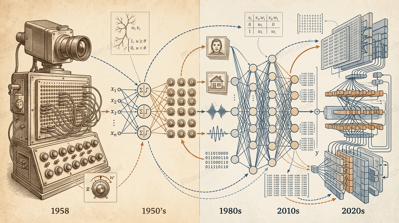
Despite these differences, the general structure remains recognizable:

1. the model receives input data;
2. it applies trainable parameters to the data;
3. it produces a prediction;
4. it compares the prediction with the desired result;
5. it calculates an error;
6. it changes the parameters;
7. it repeats the process.

The specific training algorithms have become incomparably more sophisticated, but the idea of configuring a model using data remains intact.

---

How the Perceptron Is Connected to Deep Learning

A deep neural network consists of many computational units organized into layers.

Each layer transforms information and passes the result forward.

For example, a computer vision neural network may gradually identify:

1. changes in brightness;
2. lines and edges;
3. corners and simple shapes;
4. textures;
5. parts of objects;
6. complete objects;
7. final categories.

A single perceptron cannot build this kind of hierarchy.

However, it already contains the basic structure of a trainable computational unit:

inputs → weights → sum → activation function → output.

A modern artificial neuron can be written in a similar form:

z = w₁x₁ + w₂x₂ + ... + wₙxₙ + b

y = f(z)

The differences lie in the function f, the network architecture, and the training method.

Instead of a hard threshold, modern neural networks use various activation functions:

• ReLU;
• sigmoid;
• tanh;
• GELU;
• other nonlinear functions.

Backpropagation is commonly used to modify the weights. It makes it possible to estimate the contribution of parameters not only at the output but also in the model’s internal layers.

As a result, a neural network can learn an entire sequence of transformations rather than a single linear boundary.

---

How the Perceptron Is Connected to ChatGPT and Claude

The perceptron cannot be described as a smaller version of ChatGPT or Claude.

Modern language models are based on the Transformer architecture. They process sequences of tokens, use attention mechanisms, and contain many layers with enormous numbers of parameters.

A classic perceptron:

• receives a small set of numerical features;
• performs linear classification;
• uses a threshold function;
• produces one of two answers;
• does not work with long context.

A large language model:

• processes multidimensional vector representations;
• considers relationships between tokens;
• contains many sequential layers;
• predicts probabilities for possible continuations;
• generates text, code, and other types of data.

The direct technological path between them spans decades of research into:

• multilayer neural networks;
• backpropagation;
• gradient-based optimization methods;
• deep learning;
• vector representations;
• attention mechanisms;
• the Transformer architecture.

However, the fundamental idea remains the same:

Instead of describing every rule manually, we can create a model with numerical parameters and configure it using data.

In a perceptron, the learned pattern is stored in a small number of weights. In modern AI models, it is distributed across enormous parameter matrices.

The historical connection between the Mark I, ChatGPT, and Claude therefore exists not at the level of capabilities but at the level of the general learning principle.

---

Why the Perceptron Is Still Studied

Today, the classic algorithm is rarely used to create complex AI products. More flexible methods are available for most practical applications.

Nevertheless, the perceptron remains an important part of machine learning courses.

It Clearly Demonstrates Model Training

The perceptron makes it easy to see the complete cycle:

• data;
• prediction;
• correct answer;
• error;
• parameter update;
• repeated training.

In a complex neural network, this process is hidden behind millions of calculations.

It Explains the Role of Weights

The perceptron helps demonstrate that a learned rule can be stored in numerical parameters.

A weight is not verbal knowledge. It represents the strength of a particular feature’s influence on the result.

It Explains Linear Classification

The perceptron is a useful way to study:

• decision boundaries;
• linear separability;
• classification;
• hyperplanes;
• algorithm convergence.

It Reveals Architectural Limitations

The XOR example shows that a model may fail not because it lacks data or training time, but because it cannot represent the required relationship.

It Connects History with Modern Technology

The perceptron stands between two eras:

• early mathematical models of artificial neurons;
• modern trainable neural networks.

Before the perceptron, an artificial neuron was primarily viewed as a logical element. After the perceptron, the automatic adjustment of parameters became a central idea.

---

A Brief History of the Perceptron

Year	Event
1943	McCulloch and Pitts describe a mathematical model of an artificial neuron
1949	Donald Hebb publishes a theory explaining changes in connections between simultaneously active neurons
1951	Marvin Minsky and Dean Edmonds create the SNARC neural network machine
1957	Frank Rosenblatt describes an early perceptron model
1958	Rosenblatt’s paper on the perceptron as a model for storing and organizing information is published
1958	The algorithm is demonstrated on an IBM 704 computer
1958	The Mark I Perceptron hardware system appears
1959	Rosenblatt moves his research to Cornell University’s main campus
1962	Principles of Neurodynamics is published
1969	Minsky and Papert publish Perceptrons
1980s	Interest in training multilayer neural networks returns
2010s	Deep learning becomes the foundation of many recognition and generation systems
2020s	Large neural models are widely used for text, images, code, audio, and video

---

Key Concepts

Concept	Meaning
Perceptron	A trainable threshold-based model for classifying data
Input	A numerical feature describing an object
Weight	A parameter that determines how strongly an input influences the output
Bias	A parameter that shifts the decision boundary
Weighted sum	The sum of input values multiplied by their corresponding weights
Threshold	The boundary at which the model’s output changes
Classification	Assigning an object to a particular category
Label	The correct answer for a training example
Error	The difference between the correct answer and the prediction
Learning rate	The size of the weight update during one step
Epoch	One complete pass through the training dataset
Linear separability	The ability to divide classes using a single hyperplane
Generalization	The ability to work correctly with new examples
Mark I Perceptron	Rosenblatt’s hardware implementation of a perceptron system
Supervised learning	Training on examples with known correct answers

---

Frequently Asked Questions

What Is a Perceptron in Simple Terms?

A perceptron is a simple trainable model that receives several numerical features and determines which of two classes an object belongs to. After an incorrect answer, the model changes its weights to reduce the likelihood of making a similar mistake in the future.

Who Created the Perceptron?

The perceptron was developed by American psychologist Frank Rosenblatt in the 1950s. He worked at the Cornell Aeronautical Laboratory and viewed the perceptron as a model of perception, memory, and learning.

When Was the Perceptron Created?

Rosenblatt described an early model in 1957. His scientific paper was published in 1958, and the algorithm was demonstrated on an IBM 704 computer that same year. The Mark I Perceptron hardware system also dates to this period.

What Was the Mark I Perceptron?

The Mark I Perceptron was a specialized hardware machine used for experiments in trainable image recognition. It used an array of 400 photosensitive elements, patch panels, association units, and adjustable components that represented weights.

How Does the Perceptron Learning Algorithm Work?

The perceptron receives an example, calculates an output, and compares it with the correct label. If the answer is wrong, the weights are changed according to the input values, the direction of the error, and the learning rate.

What Is a Perceptron Weight?

A weight is a numerical parameter that determines how strongly an input feature influences the final decision. The weights are automatically adjusted during training.

What Is a Bias?

A bias is an additional trainable parameter that allows the decision boundary to move. Because of the bias, the line separating the classes does not have to pass through the origin.

What Is a Single-Layer Perceptron?

It is a model without a trainable hidden layer. The input features are connected directly to an output unit through weights. This kind of perceptron creates a linear boundary between classes.

What Problems Can a Perceptron Solve?

A perceptron can solve linearly separable classification problems. For example, a simple perceptron can learn the AND and OR logical operations or separate two classes of objects when a single linear boundary can be drawn between them.

Why Can’t a Perceptron Solve XOR?

The XOR points cannot be divided using one straight line. Because a single-layer perceptron creates only a linear boundary, no suitable combination of weights exists for this problem. Solving XOR requires a hidden layer or another nonlinear transformation of the features.

Does Perceptron Training Always Succeed?

No. The algorithm is guaranteed to converge only for linearly separable data. If the classes overlap, the model may continue changing its weights without reaching a perfect solution.

Was the Perceptron the First Neural Network?

Formal neuron models and early neural network machines existed before it. However, the perceptron became one of the first widely known systems to combine a learning algorithm, a mathematical foundation, and a hardware implementation.

Is a Perceptron an Artificial Neuron?

The classic perceptron resembles a modern artificial neuron in its general structure: inputs are multiplied by weights, added together, and passed through an activation function. Modern neurons use different functions and operate as parts of multilayer networks.

Is the Perceptron Still Used Today?

The classic algorithm is primarily used in education, research, and certain linear classification tasks. For complex systems, logistic regression, support vector machines, ensemble methods, and deep neural networks are more commonly used.

How Is a Perceptron Different from Logistic Regression?

Both models create a linear boundary, but the classic perceptron uses a hard threshold function and updates its weights after classification errors. Logistic regression produces a value that can be interpreted as a probability and is trained by optimizing a continuous loss function.

How Is a Perceptron Different from ChatGPT?

A perceptron is a simple linear classifier that usually chooses one of two classes. ChatGPT is based on a multilayer Transformer architecture, processes sequences of tokens, and generates text. What they share is the idea of adjusting numerical parameters based on data.

Can a Perceptron Be Considered Artificial Intelligence?

The perceptron belongs to the history of artificial intelligence and machine learning because it can discover a classification rule from examples. However, its capabilities are extremely limited: it does not understand the meaning of data, cannot reason, and does not possess general intelligence.

---

Conclusion

Frank Rosenblatt’s perceptron became one of the most important milestones in the history of neural networks and machine learning.

The McCulloch–Pitts model demonstrated that the operation of an artificial neuron could be described mathematically. The perceptron added the next essential component: the ability to change parameters after making mistakes.

In its simplest form, a perceptron:

• receives input features;
• multiplies them by weights;
• adds the results together;
• adds a bias;
• compares the sum with a threshold;
• produces one of two answers;
• compares the prediction with the correct label;
• adjusts the weights after an error;
• gradually discovers a linear boundary between the classes.

The Mark I Perceptron demonstrated that this idea could exist as a physical, trainable machine. Its photosensitive array received an image, while adjustable components changed the state of the system during training.

The perceptron’s capabilities were limited. A single-layer model could not solve problems in which the classes could not be separated by a single linear boundary. It did not understand the content of images, was not conscious, and was infinitely far from general artificial intelligence.

But the historical importance of the perceptron is not determined by the complexity of the problems it could solve.

Rosenblatt demonstrated that a computing system could do more than execute an unchanging rule: it could form that rule from examples.

This principle remains at the heart of modern neural networks:

A model receives data, produces a prediction, evaluates its error, and changes its parameters to achieve a more accurate result next time.

Researchers later learned how to train many sequential layers, extract complex features, and work with enormous datasets. These advances led to deep learning, computer vision systems, transformers, and large language models.

The next stage in this history was the criticism of the perceptron. Researchers discovered problems that a single-layer network could not solve, regardless of how long it was trained. Inflated expectations began to give way to disappointment, and neural network research lost much of its popularity for many years.

Modern models—GPT, Claude, Gemini, and others—are incomparably more sophisticated than the perceptron. They also differ in architecture, training, fine-tuning, and optimization, which is why they may produce different answers to the same prompt.

With Riser, you can work with models from different providers in one interface, switch between them, and compare their performance on real-world tasks.

---

Continue Reading

Previous article—“The First Artificial Neuron: The McCulloch–Pitts Model”