Part 3. The First Artificial Neuron: The McCulloch–Pitts Model

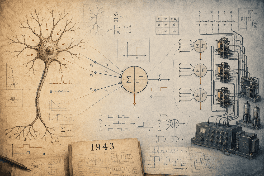
Neural networks can now generate text and images, recognize speech, analyze documents, and help people write code. Modern models may contain billions of parameters, and training them requires enormous computational resources.

However, the history of neural networks began with a much simpler idea.

Could a single brain cell be represented as a mathematical element that receives several signals, compares them with a defined threshold, and produces one of two possible outputs?

In 1943, American neurophysiologist Warren McCulloch and mathematician Walter Pitts proposed exactly such a model. Their artificial neuron could not learn automatically, process text, or create images. It accepted binary signals and returned only 0 or 1.

Despite its simplicity, this model became one of the most important theoretical foundations of future neural networks.

Quick answer: who created the first artificial neuron?

The first artificial neuron is commonly associated with Warren McCulloch and Walter Pitts. In December 1943, they published the paper A Logical Calculus of the Ideas Immanent in Nervous Activity.

The researchers represented the nervous system as a network of simple logical elements. Each element received input signals and produced an output when excitation reached a defined threshold.

The basic principle can be represented like this:

excitatory inputs of 0 or 1 → count active signals → compare with the threshold → check the inhibitory input → return 0 or 1.

This was one of the first times the biological concept of a neuron had been given a rigorous mathematical form.

In the original McCulloch–Pitts model, excitatory connections did not have different numerical weights. Every active excitatory input was counted as a single signal. At the same time, an active inhibitory input could block the neuron completely.

The weighted-sum formula appeared in later models and is now frequently used as a convenient generalization of the threshold principle.

It is important to clarify that the McCulloch–Pitts model was theoretical. It was neither the first physically constructed neural network nor the first network capable of learning from examples. Nevertheless, it became one of the major starting points in the history of artificial neural networks.

The paper was published in December 1943 in volume 5 of the Bulletin of Mathematical Biophysics, on pages 115–133.

---

Who were Warren McCulloch and Walter Pitts?

The creators of the model approached the problem from two different directions. McCulloch studied the brain and nervous system, while Pitts specialized in mathematical logic.

Their collaboration connected biology and mathematics—fields that had rarely been treated as parts of the same computational problem.

Warren McCulloch

Warren Sturgis McCulloch was an American physician, neurophysiologist, psychiatrist, and one of the future participants in the cybernetics movement.

He was interested in a fundamental question:

How does the physical activity of nerve cells produce perception, memory, reasoning, and thought?

McCulloch studied more than medicine and physiology. He was also interested in philosophy, logic, and mathematical ways of describing how the brain works.

Simply listing the components of the nervous system was not enough for him. He wanted to identify the rules through which interactions between neurons could produce complex behavior.

This approach aligned with the scientific ideas of the first half of the 20th century. Researchers already understood that the nervous system consisted of individual cells that transmitted signals. At the same time, mathematicians were developing formal logic, while engineers were learning to construct electrical circuits from switches.

McCulloch believed these fields were connected.

Walter Pitts

Walter Pitts was an American logician and mathematician. He was particularly interested in formal systems—ways of representing complex reasoning as a sequence of precise operations.

While McCulloch approached the problem from the perspective of the nervous system, Pitts could translate biological assumptions into the language of mathematical logic.

Their goal was not to create a detailed copy of the living brain. Instead, they selected several basic properties of nerve cells and used them to build an abstract computational model.

This model became known as the McCulloch–Pitts neuron.

---

What did McCulloch and Pitts propose in 1943?

McCulloch and Pitts titled their paper A Logical Calculus of the Ideas Immanent in Nervous Activity.

The title reflected their central idea: the behavior of a network of nerve cells could be described using formal logic.

The researchers based their model on several simplifying assumptions:

1. a neuron receives signals from other neurons;
2. signals may excite or inhibit it;
3. excitatory signals are combined;
4. the neuron activates only after a particular threshold is reached;
5. an active inhibitory input can block activation;
6. the output has two possible states—the neuron is either active or inactive;
7. the output of one neuron can become the input of another;
8. networks of these elements can implement logical and computational processes.

The model followed an all-or-none principle. A neuron did not produce a weak, medium, or strong response. At any given moment, it occupied one of two states:

• 0 — no signal;
• 1 — signal present.

Today, this type of construction is known as a binary threshold unit.

Another important feature of the model was discrete time. The state of the network was evaluated across a sequence of steps: signals received by a neuron at time t determined its state at the next step, t + 1.

This made it possible to describe not only individual logical operations but also networks with cycles, in which previous activity influenced future behavior.

The model’s most significant contribution was not the capability of a single artificial neuron. It was the possibility of connecting artificial neurons into networks.

McCulloch and Pitts showed that such systems could represent logical expressions and perform computations.

---

How a biological neuron became a mathematical function

A biological neuron is a complex living cell. It has dendrites, a cell body, an axon, synapses, and numerous electrochemical processes.

McCulloch and Pitts did not attempt to reproduce all these details. Instead, they created a functional simplification.

Biological neuron

At the most general level, a living neuron:

1. receives signals from other cells;
2. combines excitatory and inhibitory influences;
3. responds when activity reaches a particular level;
4. transmits a signal to other cells.

Artificial neuron

In the mathematical model, biological processes are replaced with numbers and formal rules:

1. input signals take the value 0 or 1;
2. connections are divided into excitatory and inhibitory types;
3. active excitatory signals are counted;
4. their number is compared with a threshold;
5. the model checks for inhibition;
6. the output becomes either 0 or 1.

The relationship can be illustrated in a table.

Biological element	Mathematical equivalent
Signals from other cells	Binary input values
Synaptic connections	Excitatory and inhibitory connections
Excitation of the cell	Number of simultaneously active excitatory inputs
Inhibitory influence	Input that blocks activation
Activation threshold	Defined minimum number of signals
Generation of an impulse	Output 1
Absence of an impulse	Output 0
Connections between neurons	Structure of the artificial network
Transmission of a signal over time	Transition from step t to step t + 1

Numerical weights of different magnitudes belong to later developments in artificial neuron models.

This comparison does not mean that the mathematical model is an exact digital copy of a living cell. It is better understood as a computational structure inspired by selected features of the nervous system.

---

Artificial neuron explained simply

Imagine a security system that opens a door only when two conditions are met:

• the access card is recognized;
• the correct PIN has been entered.

Each condition can be represented as a binary input:

• x₁ = 1 if the card is valid;
• x₂ = 1 if the PIN is correct.

Now set the activation threshold to 2. This means both signals are required:

x₁ + x₂ ≥ 2

Let us examine every possible combination.

Card x₁	PIN x₂	Number of active inputs	Access
0	0	0	0
0	1	1	0
1	0	1	0
1	1	2	1

The door opens only when both conditions are satisfied.

The artificial neuron in this example does not think or understand what an access card or PIN is. It simply follows a predefined rule:

if the number of active inputs reaches the threshold, return 1; otherwise, return 0.

An inhibitory input can also be added to the system. For example, if security personnel manually lock the door, access will be denied even when the card and PIN are both correct.

More complex computational systems can be built by combining many simple rules of this kind.

---

Input signals, threshold, inhibition, and output

In the original McCulloch–Pitts model, a neuron received two types of binary signals:

• excitatory signals moved the neuron toward activation;
• inhibitory signals prevented activation.

A simplified version of the rule can be written as follows:

E = x₁ + x₂ + ... + xₙ

y = 1 if E ≥ θ and no inhibitory input is active;

y = 0 in every other case.

Here:

• x₁, x₂, ... xₙ are excitatory inputs with values of 0 or 1;
• E is the number of active excitatory inputs;
• θ is the activation threshold;
• y is the neuron’s output;
• an active inhibitory input blocks the output regardless of the value of E.

For example, suppose a neuron has three excitatory inputs and a threshold of 2. It activates when at least two inputs receive a signal. However, if an inhibitory connection activates at the same time, the output remains 0.

Input signals

An input indicates whether a particular signal, feature, or event is present.

For example:

• a sensor detects movement — 1;
• no movement is detected — 0;
• a user enters the correct password — 1;
• the password is incorrect — 0.

In the McCulloch–Pitts model, inputs and outputs are binary.

Excitatory connections

An excitatory input contributes to the activation of the neuron.

In the basic model, each excitatory input is counted as one signal. If the threshold is 2, the neuron requires at least two simultaneously active excitatory inputs.

Suppose the neuron receives three signals:

E = x₁ + x₂ + x₃

With the threshold θ = 2, the results are:

x₁	x₂	x₃	E	Output with threshold 2
0	0	0	0	0
1	0	0	1	0
1	1	0	2	1
1	0	1	2	1
0	1	1	2	1
1	1	1	3	1

Inhibitory connections

An inhibitory input behaves differently. It does not simply reduce the total. Instead, it blocks the neuron’s activation.

Suppose all three excitatory inputs are active and the threshold has been reached:

1 + 1 + 1 = 3

With a threshold of 2, the neuron would normally return 1. However, if an inhibitory input is active at the same time, the result becomes 0.

threshold reached → inhibitory input active → output 0.

This principle is known as absolute inhibition.

Threshold

The threshold determines how many excitatory signals are required for activation.

For example:

• with a threshold of 1, one active input is sufficient;
• with a threshold of 2, at least two active inputs are required;
• with a threshold of 3, three inputs must activate simultaneously.

The threshold converts the number of received signals into a binary decision.

Output

The model has only two possible outputs:

• 0 — the neuron did not activate;
• 1 — the neuron activated.

The output may serve as the final result or be transmitted to other artificial neurons during the next time step.

Where do weights in modern explanations come from?

Modern textbooks usually describe an artificial neuron using a weighted sum:

S = x₁w₁ + x₂w₂ + ... + xₙwₙ

Here, the weight w determines the influence of each input. One signal can affect the output more strongly, another more weakly, while a third may receive a negative weight.

This notation is useful for explaining perceptrons and modern neural networks, but it is not a literal representation of the basic McCulloch–Pitts model.

It is therefore important to distinguish between two concepts:

• the McCulloch–Pitts neuron — a binary logical element with a threshold, excitation, and inhibition;
• the modern threshold neuron — a generalized model in which inputs may have different numerical weights.

---

A visual example of the McCulloch–Pitts neuron

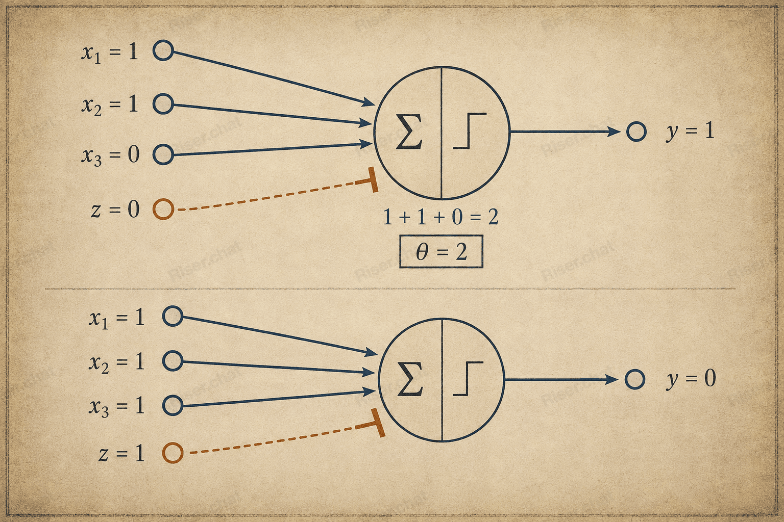
Consider a neuron with three excitatory inputs and one inhibitory input:

• x₁ = 1;
• x₂ = 1;
• x₃ = 0;
• inhibitory input z = 0;
• threshold θ = 2.

Step 1. Count the excitatory signals

1 + 1 + 0 = 2

Step 2. Compare the result with the threshold

2 ≥ 2

The activation condition has been satisfied.

Step 3. Check the inhibitory input

z = 0, so there is no inhibition.

Step 4. Get the result

y = 1

The complete process looks like this:

1 + 1 + 0 = 2 → 2 ≥ 2 → no inhibition → output 1.

Now activate the inhibitory input:

• x₁ = 1;
• x₂ = 1;
• x₃ = 1;
• z = 1.

There are enough excitatory signals:

1 + 1 + 1 = 3

However, the active inhibitory input blocks the neuron:

3 ≥ 2 → inhibitory input active → output 0.

This demonstrates an important feature of the original model: even strong excitation is not enough when absolute inhibition is active at the same time.

---

What logical operations could a McCulloch–Pitts neuron perform?

Binary values can be interpreted as logical states:

• 1 — true;
• 0 — false.

By changing the network structure and activation threshold, artificial neurons can perform logical operations.

AND operation

The AND operation returns 1 only when both inputs are equal to 1.

Configuration:

• two excitatory inputs;
• threshold θ = 2.

x₁	x₂	x₁ AND x₂
0	0	0
0	1	0
1	0	0
1	1	1

The rule is:

x₁ + x₂ → if the number of active inputs is at least 2, return 1.

This is how a system requiring two simultaneous conditions can work.

OR operation

The OR operation returns 1 if at least one input is active.

Configuration:

• two excitatory inputs;
• threshold θ = 1.

x₁	x₂	x₁ OR x₂
0	0	0
0	1	1
1	0	1
1	1	1

Only one signal is required for activation.

NOT operation

The NOT operation reverses the input value:

• if x = 0, the output is 1;
• if x = 1, the output is 0.

In the McCulloch–Pitts model, this operation can be constructed using:

• a permanently active excitatory input;
• an inhibitory connection that receives the value x.

When x = 0, there is no inhibition, and the constant excitatory signal activates the output neuron. When x = 1, the inhibitory connection blocks it.

Constant excitatory input	Inhibitory input x	Output NOT x
1	0	1
1	1	0

The structure can be represented like this:

constant excitation 1 + inhibitory input x → output NOT x.

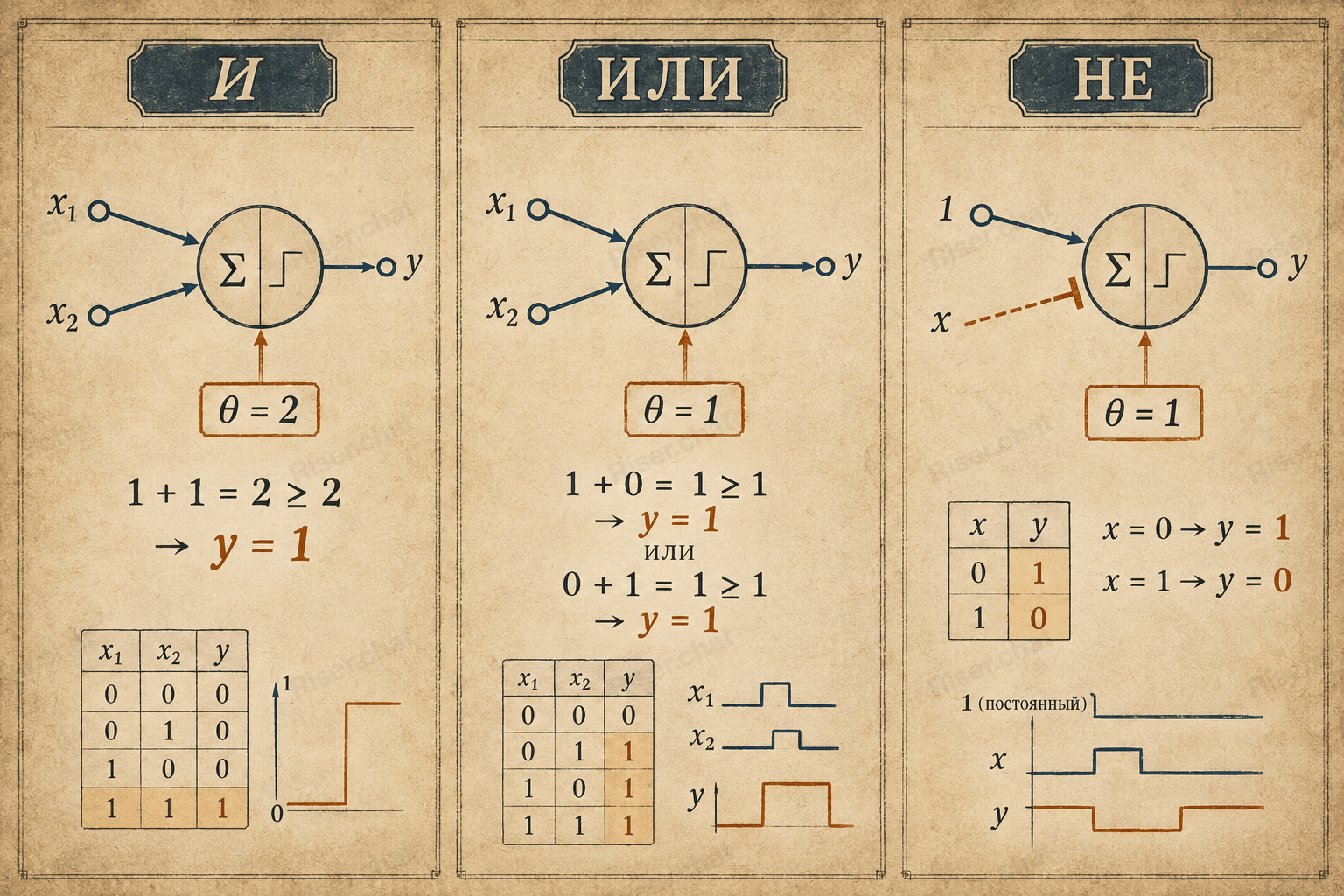
Negation is therefore implemented not simply through a negative number but through a specific structure of connections between elements in the network.

Can a neuron perform XOR?

XOR, or exclusive OR, returns 1 when exactly one of the two inputs is active:

x₁	x₂	x₁ XOR x₂
0	0	0
0	1	1
1	0	1
1	1	0

A single standard threshold unit cannot implement XOR. The reason is that these four combinations cannot be separated using a single linear boundary.

However, XOR can be constructed as a network of multiple logical elements. For example:

(x₁ OR x₂) AND NOT (x₁ AND x₂).

This reveals an important distinction:

the capabilities of a single artificial neuron are limited, while a network of several neurons can perform much more complex operations.

McCulloch and Pitts demonstrated that connecting simple elements made it possible to represent complex logical expressions.

AND, OR, and NOT form a functionally complete set, meaning their combinations can represent any Boolean function.

---

From one artificial neuron to a neural network

A single artificial neuron performs a relatively simple rule. However, its output can be directed to the input of another neuron.

Imagine the following structure:

1. the first neurons receive the initial signals;
2. each neuron evaluates its own condition;
3. the results are passed to other elements in the network;
4. additional neurons combine the received outputs;
5. the network produces the final result.

For example, a system could return 1 when the following condition is satisfied:

the object is round AND blue, but NOT small.

Several artificial neurons could be used:

• one receives the “round” feature;
• another receives the “blue” feature;
• a third receives the “small” feature;
• the next element combines the first two conditions;
• an inhibitory connection blocks the result if the object is small.

A more complex decision emerges from elementary logical operations.

The network may also contain cycles. In this case, the output of a neuron can influence future states of the system through one or more connections.

Combined with discrete time, a cyclic network gains a basic form of internal memory: its future activity depends not only on current inputs but also on previous states.

The general principle is similar to the way computer programs work. A single instruction performs a simple action, but a sequence of many instructions can produce complex behavior.

---

Could the McCulloch–Pitts model learn?

The basic formal McCulloch–Pitts model did not include an algorithm for automatic learning from examples. Connections, thresholds, and network structure were specified in advance. The model did not modify them after comparing its output with the correct answer.

However, McCulloch and Pitts did not ignore the problem of learning. Their paper discussed long-term changes in neural networks and modifiable synapses. They also showed how certain dynamic properties could be formally represented through networks containing cycles.

Still, this was not yet a practical algorithm that could automatically adjust parameters based on errors.

To create a specific network, a researcher had to define:

• the number of neurons;
• the structure of the connections;
• the excitatory and inhibitory inputs;
• the activation thresholds;
• the logical function of the network.

If the model produced an incorrect result, it could not analyze the error and restructure its own connections.

This is one of the key differences between the McCulloch–Pitts model and later trainable neural networks.

A modern model generally learns through the following process:

1. it receives an example;
2. it generates a prediction;
3. it compares the prediction with the expected result;
4. it calculates the error;
5. it changes its parameters;
6. it repeats the process across many examples.

In the basic 1943 model, connection structures and thresholds were not selected automatically from a training dataset. The network configuration required for a particular logical function had to be designed in advance.

The next major step in the development of neural networks would focus precisely on learning. In the late 1950s, Frank Rosenblatt proposed the perceptron—a system capable of adjusting its parameters in response to errors.

---

How was the model different from a real brain?

The McCulloch–Pitts model was intentionally simplified. Its purpose was not to create an exact copy of the brain but to demonstrate the computational capabilities of networks built from threshold elements.

McCulloch–Pitts model	Biological neuron
Uses binary inputs	Receives complex electrochemical signals
Has two states: 0 or 1	Activity depends on timing, firing frequency, and many other processes
Follows a fixed rule	Changes its properties through biological mechanisms
Uses an abstract threshold	The threshold depends on the state of the cell and its environment
Divides connections into excitatory and inhibitory types	Synaptic effects vary in strength and have a complex biological nature
Represents time as a sequence of steps	Biological processes unfold continuously
Has no practical learning algorithm	The nervous system has mechanisms of plasticity
Performs a formal logical function	Participates in the complex dynamics of a living system

The expression “artificial neuron” should therefore not be interpreted literally.

It is not a digital copy of a brain cell. It is a computational abstraction that preserves several general ideas:

• multiple inputs;
• combination of signals;
• excitation and inhibition;
• activation threshold;
• output signal;
• connection of elements into a network;
• changes in state over time.

---

Who created the first neural network?

The answer depends on what is meant by a neural network.

The first mathematical model

If the question refers to one of the earliest formal models of a network of artificial neurons, the key figures were Warren McCulloch and Walter Pitts.

Their 1943 paper showed that a network of abstract neurons could perform logical operations and implement computational behavior.

The first trainable neural network

If a neural network is understood as a system that changes its parameters based on examples, Frank Rosenblatt becomes one of the most important figures.

He developed the perceptron and proposed a learning algorithm that could automatically adjust parameters in response to errors.

The first physically implemented system

The McCulloch–Pitts model existed primarily as a mathematical construction. Neural networks were later implemented in electronic circuits and computer programs.

One early example of a physically implemented neural network system was SNARC, created by Marvin Minsky and Dean Edmonds in 1951. Rosenblatt’s perceptron was also implemented in hardware in the late 1950s.

The most accurate summary is therefore:

McCulloch and Pitts created one of the earliest formal models of an artificial neuron and neural network. Physical systems appeared later, while Rosenblatt developed the trainable perceptron.

---

Limitations of the first artificial neuron

By modern standards, the McCulloch–Pitts model was extremely simple.

Binary values only

Inputs and outputs could take only two values: 0 or 1.

Modern neural networks generally operate with real numbers. A value might be 0.12, −1.7, or 4.53, for example.

Fixed structure without a learning algorithm

The basic model did not automatically select connections or thresholds from data. The network configuration required for a particular logical function had to be designed in advance.

Absolute inhibition

A single active inhibitory input could completely block the neuron, regardless of the number of excitatory signals.

This was a useful mathematical simplification, but real nerve cells behave in a much more complex way.

Hard threshold

A small change in the number of signals could instantly change the output from 0 to 1.

For example, with a threshold of 2:

• one active input produces output 0;
• two active inputs produce output 1.

Modern neural networks often use smoother activation functions that are better suited to gradient-based learning.

Limitations of a single element

A single threshold neuron can solve only linearly separable problems. AND and OR are possible, while XOR requires a network of multiple elements.

Limited biological realism

Living neurons and synapses are far more complex. Their behavior depends on timing, chemical processes, firing frequency, the state of the cell, and the activity of surrounding neural tissue.

Yet the value of the model does not come from its biological accuracy.

It gave researchers a sufficiently simple object that could be described and analyzed mathematically.

---

Why did this simple model become a foundation of neural networks?

Despite its limitations, the McCulloch–Pitts model became important for several reasons.

1. It connected neurophysiology with mathematical logic

Before this work, research into the nervous system and formal logic had largely developed as separate fields.

McCulloch and Pitts showed how assumptions about nerve cells could be translated into the language of computation.

The result was a clear conceptual sequence:

nerve cell → abstract element → logical operation → computational network.

The artificial neuron could now be:

• described using formal rules;
• represented as a diagram;
• connected to other elements;
• analyzed mathematically;
• used to construct logical expressions;
• treated as part of a computational system.

2. It demonstrated the power of simple elements

A single artificial neuron can do very little. A network of neurons, however, can implement much more complex rules.

This idea remains central to machine learning:

complex behavior can emerge from interactions between large numbers of relatively simple computational elements.

3. It introduced the threshold principle

The pattern “receive signals, combine them, and apply a threshold” became a foundation for later artificial neuron models.

Researchers would eventually add:

• numerical weights;
• trainable parameters;
• bias terms;
• continuous input values;
• new activation functions;
• multilayer architectures;
• backpropagation algorithms.

However, the general structure remains recognizable:

inputs → parameters → combination → activation function → output.

4. It demonstrated the importance of network structure

McCulloch and Pitts showed that a system’s capabilities depend not only on the individual element but also on how the elements are connected.

One neuron cannot implement XOR, but a network of several neurons can. Networks with cycles can also incorporate previous states into their future behavior.

In other words, the artificial neuron matters—but so does the architecture of the entire network.

5. It prepared the way for the perceptron

Rosenblatt’s perceptron would differ from the basic McCulloch–Pitts model by gaining the ability to adjust parameters in response to errors.

Instead of requiring every rule to be constructed manually, the system could modify its behavior by learning from examples.

The artificial neuron was beginning to evolve from a predefined logical element into a trainable model.

---

From the McCulloch–Pitts neuron to modern neural networks

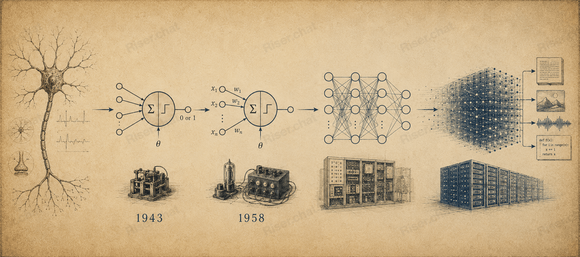
A vast technological distance separates the 1943 model from today’s large language models.

1943 model	Modern neural network
Binary inputs	Numerical vectors
Binary output	Continuous values and probabilities
Excitatory and inhibitory connections	Trainable numerical parameters
Thresholds defined in advance	Parameters selected during training
Small logical network	Enormous numbers of connected computational blocks
Hard threshold	Different nonlinear functions
No practical learning algorithm	Gradient descent and backpropagation
Simple logical tasks	Processing text, images, audio, video, and code

Modern systems such as GPT, Claude, Gemini, and other AI models are not simply enormous versions of the McCulloch–Pitts neuron. Their architectures, training processes, and mathematical foundations are far more complex.

Modern transformers also consist of more than individual artificial neurons. They use attention mechanisms, matrix transformations, normalization, multilayer blocks, and many other components.

Nevertheless, the historical and conceptual connection remains.

Computational elements in a modern network:

1. receive numerical values;
2. transform them using parameters;
3. combine the results;
4. apply a nonlinear function;
5. pass the output to other elements.

The idea of computation through a network of connected components has not disappeared. It has become substantially more sophisticated, scalable, and effective.

---

Brief timeline

Year	Event
1936	Alan Turing formalizes the concept of computation
1937	Claude Shannon connects Boolean logic with relay circuits
1943	McCulloch and Pitts publish a formal neural network model
1949	Donald Hebb describes a principle for changing connections between neurons that activate together
1951	Marvin Minsky and Dean Edmonds build the SNARC neural network machine
1957–1958	Frank Rosenblatt develops and publishes the perceptron model
1950s–1960s	Early hardware and software experiments with trainable networks appear
1980s	Practical methods for training multilayer networks become more widely used
2010s	Deep neural networks become central to image, speech, and text processing
2020s	Large neural models become widely used in generative AI

---

Key concepts

Concept	Meaning
Artificial neuron	A mathematical element that transforms input signals into an output
Binary input	A signal with a value of 0 or 1
Excitatory connection	A connection that moves the neuron toward activation
Inhibitory connection	A connection that blocks the neuron’s activation
Threshold	The minimum number of excitatory signals required for activation
Output	The neuron’s result: 0 or 1
Threshold function	A rule that converts input signals into a binary result
Discrete time	Representation of network activity as a sequence of separate steps
Neural network	A system of connected artificial neurons
Weight	A numerical value representing the influence of an input in later neuron models
Learning	The process of changing model parameters based on data and errors

---

Frequently asked questions

What was the first artificial neuron in simple terms?

It was a mathematical model that received several binary signals, counted the active excitatory inputs, and compared the result with a threshold. If the threshold was reached and no inhibition was present, the neuron returned 1. In every other case, it returned 0.

Who created the first artificial neuron?

Warren McCulloch and Walter Pitts proposed the first widely recognized mathematical model of an artificial neuron in 1943.

When did the first neural network appear?

McCulloch and Pitts described a formal model of a network of artificial neurons in December 1943. Physically implemented and trainable neural network systems appeared later.

How does a McCulloch–Pitts neuron work?

It receives binary input signals, counts the active excitatory inputs, and compares the total with a threshold. If the threshold is reached and no inhibitory input is active, the neuron returns 1. Otherwise, the output is 0.

Did the McCulloch–Pitts model use numerical weights?

In the basic model, excitatory signals were treated as equal unit inputs, while an inhibitory signal could completely block activation. Different numerical weights are characteristic of later artificial neuron models.

What is an artificial neuron threshold?

The threshold is the minimum number of excitatory signals required for activation. For example, with two inputs and a threshold of 2, the neuron activates only when both inputs are equal to 1.

How does an inhibitory input work?

An active inhibitory input blocks the neuron even when the number of excitatory signals has reached the threshold. This is one of the defining features of the original McCulloch–Pitts model.

What operations could the first artificial neuron perform?

Thresholds and different connection types could be used to implement the AND, OR, and NOT logical operations. More complex logical functions required networks of several connected neurons.

Can a single neuron perform XOR?

A single standard threshold neuron cannot implement XOR because the function is not linearly separable. However, XOR can be constructed using a network of multiple logical elements.

Could the McCulloch–Pitts neuron learn?

The basic model did not include a practical algorithm for automatic learning from examples. Its connection structure and thresholds had to be specified in advance.

The authors discussed modifiable synapses and possible changes in a network, but they did not yet provide an error-based learning algorithm.

How is an artificial neuron different from a biological neuron?

A biological neuron is a living cell involving complex electrochemical processes. An artificial neuron is a mathematical model inspired by selected features of nerve cells.

Is the McCulloch–Pitts model a perceptron?

No. The two models are historically related, but they are not identical. The perceptron appeared later and included a mechanism for changing parameters in response to errors.

Is the McCulloch–Pitts model still used today?

The original model is rarely used in modern machine learning systems. However, it is still studied as a historical foundation of threshold neurons, neural networks, mathematical logic, and computational models of the brain.

---

Conclusion

In 1943, Warren McCulloch and Walter Pitts took one of the most important steps in the history of neural networks: they transformed selected ideas about the behavior of a nerve cell into a formal computational model.

The first widely recognized formal model of an artificial neuron was remarkably simple. It:

• accepted binary inputs;
• used excitatory and inhibitory connections;
• counted active excitatory signals;
• compared their number with a threshold;
• returned 0 or 1;
• could be connected to other neurons;
• operated across sequential time steps;
• performed logical operations;
• had no practical algorithm for automatic learning.

The model’s greatest achievement was not its biological accuracy. Its real significance was that it made neural network activity mathematically describable.

McCulloch and Pitts demonstrated that complex computations could be constructed from many simple, interconnected elements.

This principle would later evolve through perceptrons, multilayer networks, deep learning, and modern generative AI systems.

The next stage was the creation of a model that could do more than follow predefined rules—it could change its parameters in response to errors. That model was Frank Rosenblatt’s perceptron.

Modern neural networks grew from the same broad mathematical foundation, but they differ dramatically in architecture, training methods, and scale. Riser lets you work with different AI models in one interface, send them the same prompts, and compare their performance on real-world tasks.

---

1. Previous article — “What Is Cybernetics? A Simple Explanation and Its Connection to Neural Networks”
   https://riser.chat/en/blog/what-is-cybernetics

2. Part 1 — “How Artificial Intelligence Began: The History of AI Before the First Neural Networks”
   https://riser.chat/en/blog/history-of-artificial-intelligence